Power Spectra and Gaussian Random Fields

This notebook will demonstrate how to generate and explore Gaussian random fields assuming a power spectrum model.

from kspace import FourierAnalysis, GaussianRandomField, PowerLawBetaModel
import numpy as np
import matplotlib.pyplot as plt

We will set up two Gaussian random fields with the same power spectrum slope, given by the PowerLawBetaModel class, which has the following functional form:

\[P(k) = C \left[1+\left(\frac{k}{k_{\rm max}}\right)^2\right]^\frac{\alpha}{2}\exp\left[-\left(\frac{k}{k_{\rm min}}\right)^2\right]\]

where \(\alpha\) is the slope of the power spectrum in the inertial range, \(k_{\rm min} = 2\pi/\ell_{\rm min}\) is the wavenumber corresponding to the minimum or “dissipation” scale, and \(k_{\rm max} = 2\pi/\ell_{\rm max}\) is the wavenumber corresponding to the maximum or “injection” scale. The normalization constant \(C\) is set to unity by default, but can be changed to achieve a desired RMS value of the field, as shown below.

# Parameters for the Gaussian random fields
l_min1 = 10.0 # minimum or "dissipation" scale for the first power spectrum
l_min2 = 30.0 # minimum or "dissipation" scale for the second power spectrum
l_max = 200.0 # maximum or "injection" scale
alpha = -11.0 / 3.0 # power-law slope in the inertial range

# Make two power spectra with different l_min values
power_spec1 = PowerLawBetaModel(l_min1, l_max, alpha)
power_spec2 = PowerLawBetaModel(l_min2, l_max, alpha)

We can now renormalize each power spectrum to have a desired RMS value using the renormalize method, which takes an RMS value as an argument and adjusts the normalization constant \(C\) accordingly, such that (assuming three dimensions and isotropy):

\[f_{\rm RMS}^2 = \int 4\pi{k^2}{P(k)} dk\]

f_rms = 10.0  # normalization of the field
# Renormalize the power spectra to have the desired RMS value
power_spec1.renormalize(f_rms)
power_spec2.renormalize(f_rms)

Next, we set up the Gaussian random field generators for the two power spectra, and generate realization of the scalar field:

# First we set up a grid
le = np.array([0.0, 0.0, 0.0])
re = np.array([750.0, 750.0, 750.0])
ddims = [256] * 3
width = re - le

# This makes a Gaussian random field with the first power spectrum
g1 = GaussianRandomField(le, re, ddims, power_spec1, seed=10)
v1 = g1.generate_scalar_field_realization()

# Make another field with the second power spectrum
g2 = GaussianRandomField(le, re, ddims, power_spec2, seed=10)
v2 = g2.generate_scalar_field_realization()

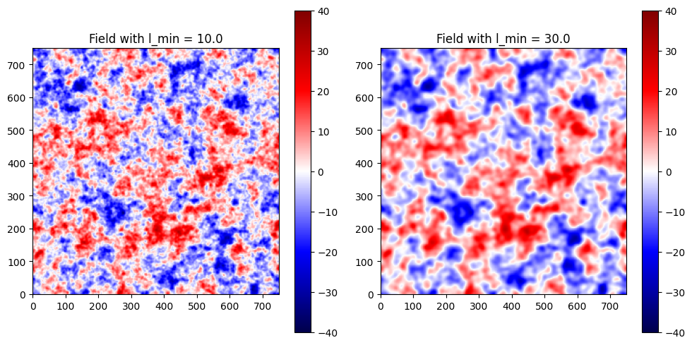
We can now plot the slices of the two fields to see the difference between them. We used the same random seed for both fields, so they should have similar large-scale structure, but the small-scale structure will be different due to the different minimum scales.

fig, ax = plt.subplots(1, 2, figsize=(10, 5))
extent = (le[0], re[0], le[1], re[1])
im1 = ax[0].imshow(
    v1[:, :, ddims[2] // 2],
    origin="lower",
    extent=extent,
    cmap="seismic",
    vmin=-40.0,
    vmax=40.0,
)
ax[0].set_title(f"Field with l_min = {l_min1}")
fig.colorbar(im1, ax=ax[0])
im2 = ax[1].imshow(
    v2[:, :, ddims[2] // 2],
    origin="lower",
    extent=extent,
    cmap="seismic",
    vmin=-40.0,
    vmax=40.0,
)
ax[1].set_title(f"Field with l_min = {l_min2}")
fig.colorbar(im2, ax=ax[1])
plt.tight_layout()
plt.show()

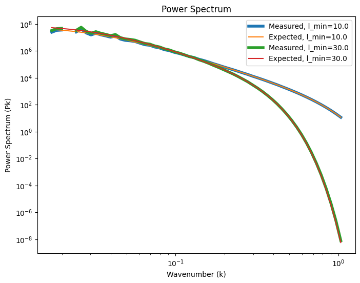
Now we can take the actual power spectra of both fields and compare them to their input power spectra. First, we create an instance of the FourierAnalysis class, which will help us with these tasks.

# Give the FourierAnalysis class the same width and dims as
# the GaussianRandomField created above
fa = FourierAnalysis(width, ddims)

We can compute the power spectra here:

nbins = 60  # Number of bins for the power spectrum, it will
# use the min-max wavenumbers as boundaries
kbins1, Pk1 = fa.make_binned_powerspec(v1, nbins)
kbins2, Pk2 = fa.make_binned_powerspec(v2, nbins)

and plot them against the expected power spectra from the PowerLawBetaModel class.

# Take the geometric mean of the bins since they are logspaced
k1 = np.sqrt(kbins1[1:]*kbins1[:-1])
k2 = np.sqrt(kbins2[1:]*kbins2[:-1])

# Now let's plot both the expected and computed power spectra
fig, ax = plt.subplots(1, 1, figsize=(8, 6))
ax.loglog(k1, Pk1, label=f"Measured, l_min={l_min1}", lw=4)
ax.loglog(
    k1, power_spec1(k1), label=f"Expected, l_min={l_min1}"
)
ax.loglog(k2, Pk2, label=f"Measured, l_min={l_min2}", lw=4)
ax.loglog(
    k2, power_spec2(k2), label=f"Expected, l_min={l_min2}"
)
ax.set_xlabel("Wavenumber (k)")
ax.set_ylabel("Power Spectrum (Pk)")
ax.set_title("Power Spectrum")
ax.legend()

<matplotlib.legend.Legend at 0x10ed20830>