Vector Field Decomposition

This example shows how to generate a Gaussian random vector field and decompose it into its compressive (divergence) and solenoidal (curl) components. It also computes the power spectra of these components and performs some sanity checks to verify the decomposition.

from kspace import FourierAnalysis, GaussianRandomField, PowerLawBetaModel
import numpy as np
import matplotlib.pyplot as plt

First, set up the power spectrum model:

# Parameters for the power spectrum
l_min = 30.0
l_max = 200.0
alpha = -11.0 / 3.0
f_rms = 10.0  # normalization of the field

# Make a power-law spectrum
power_spec = PowerLawBetaModel(l_min, l_max, alpha)

# Renomalize the power spectrum to have the desired RMS value
power_spec.renormalize(f_rms)

Next, we set up the Gaussian random field generator, and generate a realization of the vector field:

# Parameters for the box and grid
le = np.array([0.0, 0.0, 0.0])
re = np.array([750.0, 750.0, 750.0])
ddims = [256] * 3
width = re - le

# Generate a gaussian random vector field
vgen = GaussianRandomField(le, re, ddims, power_spec, seed=10)
v = vgen.generate_vector_field_realization()

v is now a 3D vector field in the form of a NumPy array, with shape (3, 256, 256, 256), where the first dimension of the array corresponds to the three components of the vector field. Now, we can decompose the field into its compressive and solenoidal components, and compute their power spectra. First, we create an instance of the FourierAnalysis class, which will help us with these tasks.

# Give the FourierAnalysis class the same width and dims as
# the GaussianRandomField created above
fa = FourierAnalysis(width, ddims)

# Decompose the field into its compressive (divergence) and solenoidal components
vc = fa.divergence_component(v)
vs = fa.solenoidal_component(v)

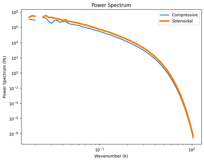
Now that we have the compressive and solenoidal components of the vector field, we can compute their power spectra and plot them:

nbins = 60  # Number of bins for the power spectrum, it will
# use the min-max wavenumbers as boundaries
kc_bins, Pkc = fa.make_binned_powerspec(vc[0], nbins)
ks_bins, Pks = fa.make_binned_powerspec(vs[0], nbins)

# Take the geometric mean of the bins since they are logspaced
kc = np.sqrt(kc_bins[1:]*kc_bins[:-1])
ks = np.sqrt(ks_bins[1:]*ks_bins[:-1])

fig, ax = plt.subplots(1, 1, figsize=(8, 6))
ax.loglog(kc, Pkc, label="Compressive", lw=2)
ax.loglog(ks, Pks, label="Solenoidal", lw=4)
ax.set_xlabel("Wavenumber (k)")
ax.set_ylabel("Power Spectrum (Pk)")
ax.set_title("Power Spectrum")
ax.legend()

<matplotlib.legend.Legend at 0x111896660>

Now, let’s do some sanity checks.

# Compute the velocity magnitude field for the following sanity checks
vmag = np.sqrt(np.sum(v*v, axis=0))

For a gaussian random field in 3D, 1/3 of the power should be in compressive motions and 2/3 should be in solenoidal, let’s check it:

print("Fraction of power in compressive motions: ", np.sum(vc*vc)/np.sum(vmag**2))
print("Fraction of power in solenoidal motions: ", np.sum(vs*vs)/np.sum(vmag**2))

Fraction of power in compressive motions:  0.3336281924898164
Fraction of power in solenoidal motions:  0.6663718075101835

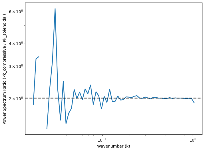
We can also check this by dividing the solenoidal power spectrum by the compressive power spectrum, which should be \(\approx\) 2. We can plot it:

fig, ax = plt.subplots(1, 1, figsize=(8, 6))
ax.loglog(kc, Pks/Pkc, lw=2)
ax.axhline(2.0, ls="--", color="k", lw=2)
ax.set_xlabel("Wavenumber (k)")
ax.set_ylabel("Power Spectrum Ratio (Pk_compressive / Pk_solenoidal)")

Text(0, 0.5, 'Power Spectrum Ratio (Pk_compressive / Pk_solenoidal)')

Similarly, the solenoidal field should be divergence-free. We can take its divergence and check that it is small compared to the magnitude of the field. Since v (and therefore vs) comes from an FFT-generated, periodic field, we pass periodic=True so the finite-difference divergence uses wraparound differences at the domain edges, consistent with the periodic (Fourier-space) projection that produced vs – otherwise the one-sided differences divergence_of_field uses by default at the boundary (appropriate for general, non-periodic data) would show up as a spurious residual there.

div_vs = fa.divergence_of_field(vs, periodic=True)
print(np.abs(div_vs*fa.delta[0]/vmag).mean())

1.2807221551813742e-16

The same goes for the compressive component, which should be curl-free (again passing periodic=True for the same reason):

curl_vc = fa.curl_of_field(vc, periodic=True)
print(np.abs(curl_vc*fa.delta[0]/vmag).mean())

7.171739745857824e-17